As mentioned half a year ago, apart from data structure rearrangement, thread divergence reduction, we can also optimize the SIMD performance by doing thread compaction. The first section below will introduce how I figure it out using the CUDA Thrust API, followed by a proposition of a new method for parallel construction of kd-tree on GPU.
The following sections will introduce three types of optimizations based on CUDA architecture – data structure rearrangement, thread divergence reduction and thread compaction used in our path tracer to increase the SIMD efficiency and reduce the overall rendering time. The necessity of most of these optimizations comes from the real-time rendering requirement, without the possibility to design fixed number of samples for each rendering branch. After that, two sections will be dedicated to discussion of optimizations on specific components - a ray-triangle algorithm better for SIMD performance will be introduced and
11.1 Thread Compaction
Russian roulette is necessary for transforming the theoretically infinite ray bounces to a sampling process with finite stages, which is terminated by probability. While decreasing the expected number of iterations for each thread in every frame and causing an overall speedup due to early terminated thread blocks, it scatters terminated threads everywhere, giving a low percentage of useful operations across warps (32 threads in a warp are always executed as a whole) and an overall low occupancy (number of active warps / maximum number of active warps) in CUDA, which aggravates as number of iterations increases.
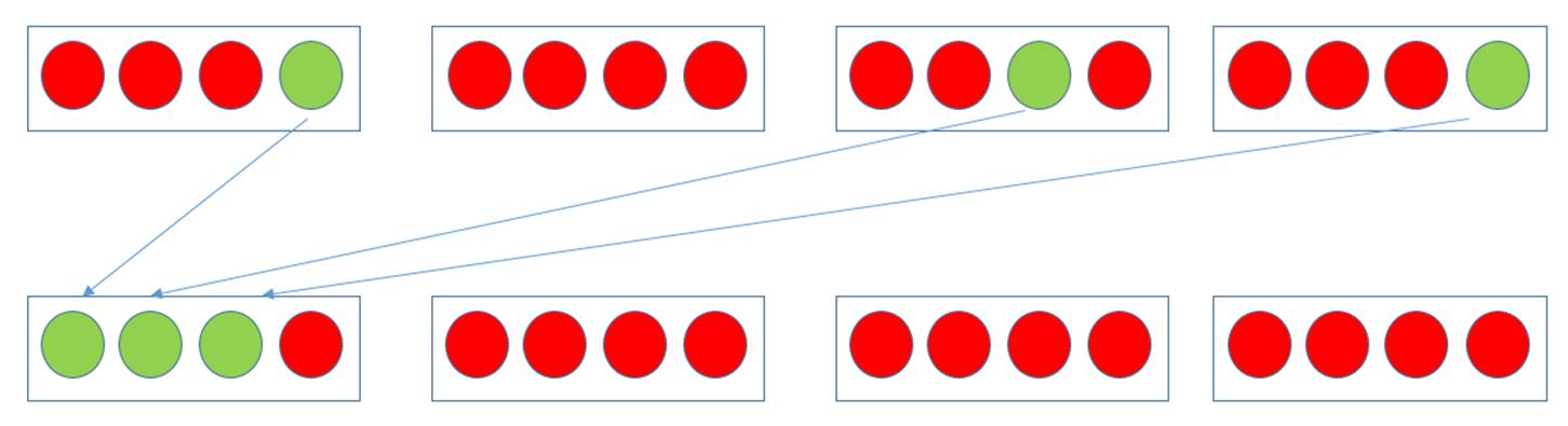
Relating to the set of basic parallel primitives, one naturally finds that stream compaction on the array of threads is very suitable for solving this problem. As illustrated in Figure 16, assuming each warp only contains 4 threads and there is only one block with 4 warps running on GPU for simplification and using green and red colors to represent active and inactive threads, before stream compaction the rate of useful operations is 25% (3 active threads out of 12 running threads) and after grouping the 3 active threads to a same warp, the percentage of useful operations becomes 75%, equivalently, same amount of work can be done by 1/3 amount of warps, leaving space for other blocks to execute their warps. Also, if the first row is the average case for multiple blocks, the occupancy would be 75% since each block with 4 warps has an inactive warp, implying that less amount of work can be done with same amount of hardware resources. With stream compaction, occupancy is close to 100% in first few iterations, before the time when total number of active threads is not enough to fill up the stream multiprocessor.
In order to measure the performance impact of thread compaction, we designed a test comparing frame rate of path tracing with and without thread compaction on our NVIDIA GeForce GTX 960M for maximum trace depth from 1 to 10, and 20, 50, 100. The test scene is the standard Cornell box rendering with next event estimation with 1,048,576 paths traced in each frame.
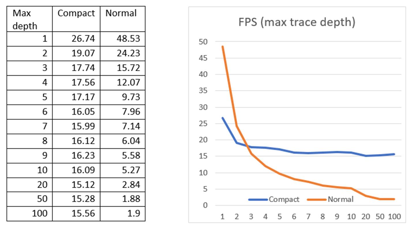
As shown by Figure 17, without thread compaction, the frame rate experiences a rapid decline in first 5 increments of max trace depth, after which the declination of frame rate approximates a linear function until the depth when all threads become inactive probably between 20 and 30. With thread compaction, the frame rate starts to surpass the original one in depth 3 with only little falloff for every depth increment and become almost stable after depth 5.
The reason thread compaction causes first two max depths slower is that thread compaction has some overhead of initialization, which cannot be offset by the speedup provided by stream compaction when terminated threads are too few. A struct stores next ray, mask color, pixel position and state of activeness needs to be initialized at the beginning for each thread and retrieved in every bounce. For stream compaction, we also use Thrust library introduced in Chapter 2, which offers a remove_if () function to remove the array elements satisfying the customized predicate. For this task, the customized predicate takes the struct as the argument and checks whether the state of activeness is false to determine elements to discard.
Nevertheless, we can also use stream compaction to do a rearrangement of threads such that threads that will be running the same Fresnel branch in next iteration are grouped together. The number of stream compaction operations will be equal to the number of Fresnel branches (which in our case is 3). By using double buffering, the results of stream compaction can be copied or appended to another array. After generating the resorted array, the indices for the buffers are swapped. In our experiment with a simple scene adapted from the Cornell box with glossy reflection, diffuse reflection and caustics, up to 30% speedup can be achieved from regrouping the threads.
11.2 GPU SAH Kd-tree Construction
We will propose a GPU SAH kd-tree construction method in this section. So far, the CPU construction of SAH kd-tree has a lower bound of O(N log N), which is still too slow for complex scenes with more than 1 million triangles. It takes more than 10 seconds to construct the SAH kd-tree for the 1,087,716-face Happy Buddha model on our Intel i7 6700HQ, which is a serious overhead. Given the immense power of current GPGPU, it is a promising task to adapt the kd-tree construction to a parallel algorithm. A GPU kd-tree construction algorithm was proposed by Zhou et al. (2008), which splits the construction levels into large node stages where median of the node’s refitted bounding box is chosen as the spatial split the and small node stages where SAH is used to select the best split. Although with a high construction speed, the method sacrifices some traversal performance due to the approximated choice of best splits in large node stages. In contrast, we will now propose a full SAH tree construction algorithm on GPU.
First, similar to Wald’s CPU kd-tree construction model (2006), we create an event struct containing the 1D position, type (0 for starting event, 1 for ending event), triangle index (which is actually triangle address since at the beginning the node-triangle association list is same as the triangle list), and a “isFlat” Boolean which marks whether the opposite end has the same coordinate for every end of bounding boxes of triangles in all 3 dimensions, which are stored in 3 arrays. For each dimension, the event array is sorted by ascending position coordinate while keeping ending events before starting event when the positions are same (we use the same routine as in the Wald’s algorithm – subtracting the triangle of ending event from the right side before SAH calculation and adding the triangle of starting event to the left side after the SAH calculation, which can guarantee that triangles with an end lying on the splitting plane can find the correct parent – except for being parallel). Such sort should be a highly efficient parallel sort like the parallel radix sort.
After that, we separate the struct attributes into a SoA (structure of arrays) for better memory access pattern. Also, we need to create an “owner” array of length of number of triangles, which is initialized to zeros as root has an index of 0, to store the index of owner node, since we will be processing the nodes in parallel. So far, we have three position arrays, three type arrays, three triangle address arrays, three isFlat arrays, and one owner array, each of which has the same length of events from all nodes in current construction level. Nevertheless, we also need an array for node-triangle association, which lists the indices of triangles associated with nodes in current level in node-by-node order. Again, this node-triangle association list (which will be called triangle list for short) also needs an owner list, which we call “triOwner”, also initialized to zeros.
What still left for initialization are the two dynamic arrays – nodeList for storing all the processed nodes, which are pushed into as groups from the working node array of current construction level, linearly and leafTriList for storing all the triangles in leaves in leaf-by-leaf linear order.
After all initializations are done, we choose a dimension with the largest span in the root’s bounding box. Note that the selection of such dimension will be processed in parallel in following iterations, at the moment of creating node structs for all newly spawned children from the current level. The following explanation will treat the current construction level a general level with many nodes other than level 0. The first parallel operation other than sorting we perform is the inclusive segmented scan on the type array, the purpose of which is to count the number of ending events before the current event (or including the current event if it is an ending event) for use in the following calculation of number of triangles on the left and right side of the splitting plane, alongside with the surface areas of bounding boxes of the potential left child and right child, as is required to calculate the SAH function. In this segmented scan, the owner array is used as a key to separate events from different nodes. It is worth mentioning that for SAH calculation, the offset of the node’s events in the event list is stored in the node struct, so that an event is able to know its relative position in its belonging part in the array, which will be used together with the scanned result of number of starting events to the left to derive the number of triangles in the left or right subspace of the splitting plane. For SAH calculation for splitting plane with flat triangle lying on it, we simplified the process by grouping all such flat triangles to the left side, which in most cases has no influence on traversal performance, so that we do not need to deal with the flat case specially in triangle counting. The information of a potential split is stored in a struct containing SAH cost, two child bounding boxes, splitting position, and number of left side and right side triangles. The array of such struct then undergoes a segmented reduction to find the best split (with minimal SAH cost) for each node.
The next step is assigning triangles to each side, which is also the step where we determine whether to turn the interesting node to a leaf. In the assigning function which is launched for every event in current splitting dimension in parallel, we check whether the best cost is greater than the cost of not splitting (which in most cases is proportional to the number of the triangles in the node) or the number of triangles in the node is below a threshold we set. If it is the case, we create a leaf by marking the “axis” attribute in the node struct with 3. For assigning triangles to both children, our key method is to use a bit array of twice the size of the current triangle list and let the threads of current events to assign 1 at the address at the belonging side (or two sides if the triangle belongs to both left and right side), after which the bit array is scanned to obtain the address of the triangle list in next level. Since the events are in sorted order, an event can decide its belonging by comparing the index with the index of the event chosen for best split. If the event is a starting event, and index is smaller than the best index, the event will assign its triangle to the left side; and if the event is an ending event, and the index is greater than the best index, the event will assign its triangle the right side. Notice that because we are launching a thread for each event, a triangle spanning across the splitting plane will be correctly assigned to both side by different threads, without special care. In addition, flat triangles lying on the splitting plane will be assigned to both sides (where isFlat variable is checked) to avoid the effect of numerical inaccuracy in traversal which can cause artefacts.
Also, a leaf indicator array is assigned by the threads in the triangle assignment function such that the indicator array would have a 1 in the position of triangles that belong to a newly created leaf in the triangle list, which will be scanned to determine the address of the triangle in the leafTriList, similar to how the addresses of triangles in the next level’s triangle list are determined, and reduced to obtain the number of triangles in the leafTriList in current level which is used to calculate the new size of the whole leafTriList to be used as next level’s offset. Since we also need to know the local offset of the leaf’s triangles in the part of current level in leafTriList, we need to do a segmented reduction followed by an exclusive scan on the leaf indicator array before assigning the offset to the leaf’s struct.
Before spawning new events for the child nodes, we need to finish the rest of the operations on the triangle list. The triOwner list for the new level can be easily generated by “spawning” a list from the original triOwner list with doubled size by appending the list to itself with the owner index offset by the original number of owners of nodes in the second half and performing a stream compaction using the aforementioned bit array as the key to remove the entries for triangle not belonging to the specific side. A question may be that after the stream compaction, the owner indices are not incremental, which cannot be used for indexing. However, this issue can be easily solved by doing a parallel binary search on the returned key array of the segmented reduction (or counting, more properly) on the constant array of 1 (the returned value array of which is stored as the counts of the triangles in next level’s nodes) with the just generated next level’s triOwner array itself as the key, whose result is used to replace the array. In a similar way, the triangle list for next level is “spawned” from the original triangle list and compacted by the bit array.
Finally, we explain how the next level’s events (type, split position, isFlat and triangle address) are generated. The method is surprisingly simple – after duplicating the event list, we only need to produce a bit array for events by checking the corresponding values in the bit array for triangles, which only requires reading the values in current events’ triangle address list as the pointer to the position in the bit array for triangle. The 3 attributes type, split position and isFlat can be spawned by duplicating the original array and perform a stream compaction with the bit array as the key. The triangle address array itself can spawn the array for next level by duplicating, reading the new addresses in the previously scanned result of the triangle bit array and also doing a stream compaction.
So far, there is only one last array to spawn – the event’s owner list in the next level, which can be generated in the same method as the triOwner array uses – “stream compaction – segmented reduction – binary search”. Before next iteration begins, node structs for next level are created using data like counts and offsets in the corresponding previous generated arrays and pushed to the final node list as a whole level. The splitting axes for the next level are also chosen in this process by comparing the lengths of the 3 dimensions of the bounding box. If an axis different from current axis is chosen, the 4 event arrays for the 3 dimensions are “rotated” to the desirable place – if 0 stands for the splitting axis and current splitting axis is x, y and z will be stored under index 1 and 2; if next splitting axis is z, the memory will have a “recursive downward” rotation so that z is rotated to 0, x is rotated to 1, y is rotated to 2. Finally, the pointers of all working arrays are swapped with the buffered arrays. The termination condition is that the next level has no nodes.
We also performed a test comparing the speed between Wald’s CPU construction and our GPU construction of the same SAH kd-tree (full SAH without triangle clipping) on a computer with Intel i7-4770 processor and NVIDIA GTX 1070 graphics card. The result (Table 2) shows that a sufficiently large model is required for our GPU construction to outperform the CPU counterpart, due to the overhead of memory allocation and transfer. A 5x speedup can be obtained when the model size goes beyond 1M, which indicates that our method can be used for ray tracing large models to greatly reduce the initialization overhead while maintaining the same tree quality.
| Model | Face Count | CPU(s) | GPU(s) | Speedup |
|---|---|---|---|---|
| Cornell | 32 | 0.001 | 0.046 | 0.02x |
| Suzanne | 968 | 0.016 | 0.095 | 0.17x |
| Bunny | 69,451 | 1.442 | 0.655 | 2.20x |
| Dragon | 201,031 | 3.705 | 1.100 | 3.37x |
| Buddha | 1,087,716 | 13.903 | 2.801 | 4.96x |