3.1 The Rendering Equation
The rendering equation introduced by Kajiya (1986) defines the radiance seen from a point  in the reflection direction
  , i.e. view vector in ray tracing’s grammar as a result of reversibility of light path:
 which is the emittance of the point itself plus the reflectance caused by all incident radiance summed from the surrounding hemisphere. This is a physically correct model of global illumination considering only surface to surface reflection. In computer graphics, this is usually mapped into a recursion where the integral is decomposed into randomly picked samples. For path tracing, all possible light paths from the set of light rays within a pixel are sampled individually from random position within the pixel whose results are then averaged. Upon hitting a surface, only one secondary ray is shot for each sample. It intuitionally follows that the secondary ray must be generated with some probability mechanisms, which is defined by BRDF
  with respect to the surface property. However, there are some problems. Given limited number of samples, how do we choose a proper sampling strategy to maximize the image quality? Given a specific BRDF, how to translate it into an algorithm that fits into the sampling strategy we use?
3.2 Stratified Sampling vs. Anti-aliasing Filters
To generate samples within pixels, a naïve solution is uniform sampling. In CUDA device code, the function curand_uniform(seed) can generate 1D uniform pseudorandom samples from 0 to 1. However, the uniformly distributed samples tend to form clusters, producing high noise level. A common way to overcome this is stratified sampling, which divides a pixel into  grids and takes uniform samples of same number within each grid. Theoretically, it reduces the error of estimation from
  to
to  , where n is the number of samples. A problem of stratified sampling is that it is not suitable for successive refinement required in real-time rendering. When using successive refinement, usually one sample is taken for every pixel in each frame. If we want to have minimum aliasing effect in any given frame, the former samples must at least not follow any certain fixed pattern, which is not possible for stratified sampling which must use at least samples as a unit. Therefore, we want to find a solution having both low noise level and successive refining capability.
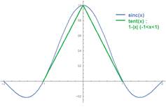
In the famous 99 lines of C++ implementation of path tracing SmallPT, Beason (2007) applies a tent filter to the uniform random samples which shift more samples towards the center of the pixel. In my test, this method produces same image quality given same sampling number as stratified sampling does with the ability of successive refinement. In fact, it approximates the sinc function, the ideal anti-aliasing filter (Figure 3). There are actually other choices of approximation with higher quality such as bicubic filter and Gaussian filter. However, these filters have much higher computation overheads while the tent filter is a more practical choice in real-time rendering.
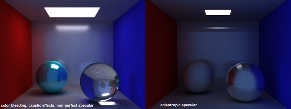
Sample rays reflected by the surface can be chosen from all possible directions within the hemisphere of the incident point. Without using importance sampling, it is hard to achieve a reasonable convergence rate when the variance of radiance is high enough. Consider two factors: surface characteristics and spatial distribution of incoming radiance. The first factor can be easily described by BRDF models that offers distribution function for importance sampling. In contrast. the second factor is more difficult to analyze. For cases that light comes directly hitting the surface such as diffuse reflection, references to emitting surfaces (lights) can be stored separately to enable explicit light sampling. However, when transmission is included, this method no longer works. Effects like caustics must be achieved using bi-directional path tracing, if importance sampling with respect to incoming radiance distribution is required. This is a topic I planned to study in the next half of project.
3.3 BRDF & Anisotropic Material
For importance sampling based on BRDF, an important progress I have achieved is the simulation of anisotropic material. Ward (1992) introduced a practical BRDF by modifying the Beckmann distribution factor in Cook-Torrance Model (1982),
where  and
and  correspond to “roughness” of the material in x and y direction w.r.t. tangent space. Taking azimuth angle
  as argument, it is easy to see that when
  the distribution is completely determined by and when
  the distribution is totally decided by . However, in my implementation of anisotropic materials I chose GGX function instead of Beckmann function due to its simplicity and faster computation. An isotropic version of GGX was adopted in Unreal Engine 4 (Karis, 2013):
By replace  with
with  , the equation works for anisotropic surfaces. It turns out that the sampling azimuth angle and altitude angle
  can be computed with
 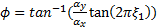 and
and 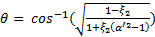 , where
  and
and  are two unit uniform random variables. Notice that this result in
  , which can be computed faster than
  in Beckmann’s case, where two extra math functions cos() and log() are involved. Below is a sample picture (Figure 4) showing the anisotropic effect produced by the modified Ward model with GGX distribution.
3.4 Next Event Estimation
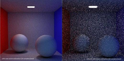
In order to utilize spatial distribution of incoming radiance in importance sampling, I applied next event estimation implemented by explicit light sampling. As mentioned before, reference to triangles with emittance greater than 0 (“light triangles”) are stored in an array. When ray hits a surface, shadow rays are shot from the hit point to every light triangle. Notice that more shadow rays imply faster convergence but lower frame rate due to extra kd-tree traversal and ray-triangle intersection cost. When doing real-time path tracing, one can determine the balance between convergence rate and frame rate heuristically.
To sample shadow rays, an end point is picked randomly within the boundary of every light triangle, which is then subtracted with the fixed start point to derive the ray direction. However, for importance sampling, the probability distribution function (pdf) needs to divide all other terms. For triangle, it is determined by the solid angle it spans w.r.t. the hit point divided by the hemispherical solid angle ( ). To compute this solid angle, an elegant formula was found by Oosterom and Strackee (1983):
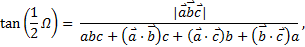
where  are the position vectors of the three triangle vertices w.r.t. to the origin.
If we normalized the three position vectors in advance, the formula is simplified to

which is more convenient for computation.
An important notice is that the triangles used for explicit lighting sampling must be excluded in the scene intersection of next ray to avoid repetitive summing of radiance. A bitmap can be used here to mark which light triangles have been explicitly sampled if the number of light triangles is within a proper limit. If it turns out that the intersected triangle was explicitly sampled in former ray, the ray will be abandoned.
Next event estimation is crucial for increasing the convergence rate for scene of high dynamic range. For example, the light’s emittance factors can be 100 times greater than the surface reflectance factors while the area of light is small. Below (Figure 5) is an example showing the significant reduction of noise level by NEE given same number of successively refined frames.
3.5 The Russian Roulette Algorithm
So far, all possible surface-to-surface reflection and refraction types are supported in my path tracing program. Russian roulette is used here to determine which type of light path to take. Apart from the diffuse color and specular color, I also defined 4 extra material parameters - transparency metalness and roughness ranging from 0.0 to 1.0, which plays the role of threshold in Russian roulette. For every ray hit, the transparency value is tested against first to determine the chance of transmission/reflection. If the transparency value is 1.0, the uniform random variable  will always be smaller or than or equal to it, branching to the transmission case. If
  , it is tested against the metalness value to determine the ratio between specular and diffuse reflection. If
  , the next ray will be generated from diffuse BRDF (lambert in my implementation). Otherwise, the next ray will be treated as the incoming radiance of a specular BRDF. Roughness is a 2D float vector, which determines the and parameters in Ward model, which will be reduced to Cook-Torrance model when two roughness values are same.
References
Beason, K. (2007). smallpt: Global Illumination in 99 lines of C++. Retrieved from http://www.kevinbeason.com/smallpt/
Cook, R. L., & Torrance, K. E. (1982). A reflectance model for computer graphics. ACM Transactions on Graphics (TOG), 1(1), 7-24.
Kajiya, J. T. (1986, August). The rendering equation. In ACM Siggraph Computer Graphics (Vol. 20, No. 4, pp. 143-150). ACM.
Karis, B. (2013). Real shading in unreal engine 4. part of ACM SIGGRAPH 2013 Courses.
Van Oosterom, A., & Strackee, J. (1983). The solid angle of a plane triangle. IEEE transactions on Biomedical Engineering, 2(BME-30), 125-126.
Ward, G. J. (1992). Measuring and modeling anisotropic reflection. ACM SIGGRAPH Computer Graphics, 26(2), 265-272.