Benchmarking different path tracing engines is not a trivial task. Different engines have different strengths at different types of rendering tasks. In addition, rendering methods may be different for different engines, thus it is difficult to choose a measure of the performance. If one engine uses Metropolis Light Transport and another engine uses brute force path tracing, one cannot claim that the first engine has a better performance than the second one, just because it has a larger frame rate (or samples per second for offline path tracing). Normally, we compare the performance by convergence rate – in same amount of time, the engine converges more has a better performance – measured by the variance level. A special reminder is that one can only use the variance measure when the engines use same basic sampling method – the only two we introduced before are normal Monte Carlo sampling and Markov Chain Monte Carlo sampling (used only in MLT) – as MLT will always try to find a smallest variance even if the color is incorrect (also known as start-up bias). Alternatively, it seems that one can also compare the absolute difference between the rendered image and the ground truth. However, the BSDF used in different engines are usually slightly different, in case of which the absolute difference is an invalid measure. A practical solution of this issue is to force different engines use the same basic sampling method (in most cases it can be changed in options) and compare the convergence rate. It is important to notice that images generated by different engines must all be tone mapped or non-tone mapped before a variance comparison can be done. Or if it is known that the engines to be compared use the same specific sampling method (like next event estimation or bi-directional path tracing), it is simpler to directly compare the frame rate. However, one should also look at the differences between the rendered image and the ground truth to prevent some low-quality images or artefacts produced by incorrect implementation or the deviation from the industrial standard.
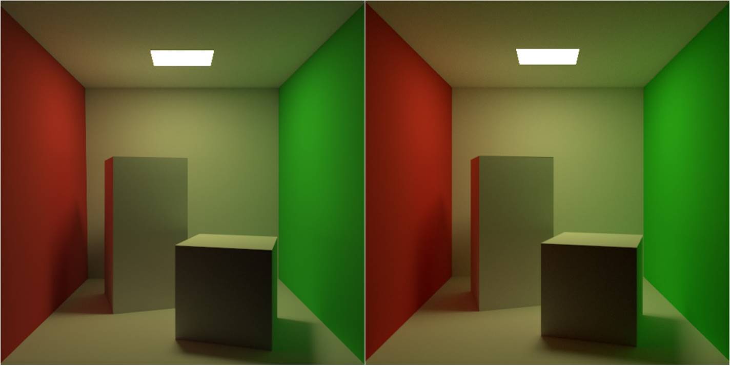
Two scenes are used to benchmark our path tracer against some free mainstream path tracers. The first scene is the default Cornell Box with all Lambertian diffuse surfaces and a diffuse area light, rendered by next event estimation. The real-time path tracing sample program of NVIDIA’s Optix ray tracing engine is used to compare with our path tracer (Figure 18). Since the sample program is open-source and uses the same next event estimation method and both our program and NVIDIA’s program are real-time path tracers, we can compare the performance by directly comparing the frame rate of rendering. Table 3 shows the frame rate of rendering of our path tracer and NVIDIA’s path tracer in 512x512 resolution with 4 samples taken for each pixel in each frame (Figure 18), on the mid-end NVIDIA GeForce GTX 960M graphics card and the high-end NVIDIA GeForce GTX 1070 graphics card.
| Type | GTX 960M | GTX 1070 |
|---|---|---|
| NVIDIA’s Path Tracer | 13.52 fps | 30.0 fps |
| Our Path Tracer | 14.02 fps | 41.5 fps |
| Speedup | 3.7% | 38.3% |
A reason for our path tracer to gain a larger speedup on high-end graphics card is that high-end graphics cards have larger memory bandwidth, which allows faster memory operations in stream compaction used in our path tracer but not in NVIDIA’s path tracer.
The second scene is the BMW M6 car modeled by Fred C. M’ule Jr. (2006), which aims for testing the capability of our path tracer to render models in real application. For comparison, we chose the Cycles Render embedded in the Blender engine. Albeit being an off-line renderer, it also has a “preview” function to progressively render the result in real-time. Notice that Cycles Render uses a different workflow to blend the material color and may use different BSDF formulae on same material attribute, causing the appearance to be different (the glasses and metal rendered by Cycles is less reflective on same attributes, and the overall tone is different). It is extremely hard to tune the rendering result to the same, but we can still guarantee that the workload on each path tracer is almost the same, as the choice of material component depends on the Fresnel equation.
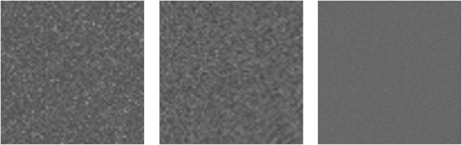
Since the ways of implementation may also be vastly different, we use the convergence rate in one minute as the measure of the performance. It is important to know that it is invalid to use the variance of all pixel in the picture to compare for convergence. As convergence corresponds to noise level in Monte Carlo sampling, a small region that will be rendered to a uniform color is used for convergence test. For this scene, it is convenient to just choose the upper-left 64x64 pixel to compare for variance, as the wall has a uniform diffuse material which will produce nearly same color under current lighting condition. Also, the rendered result of one hour from our path tracer is used as the ground truth for variance comparison (it is equivalent to use either side’s). For illumination, a 3200x1600 environment map for a forest under sun is used.
The following images in Figure 19 are the grey scale value of the upper-left 64x64 square region from Cycles Render, our path tracer, and the ground truth. By only looking with the eyes, one is difficult to judge which of our result and Cycles’ result has a lower noise level. However, we can numerically analyze the variance by evaluation of the standard deviation of the pixel values. By using OpenCV, the average value and the standard deviation of all grey scale pixels can be easily obtained, which are listed in Table 4.
| Type | Average | Std. Deviation | Convergence |
|---|---|---|---|
| Theirs | 98.42 | 10.31 | 16.7% |
| Ours | 98.95 | 9.41 | 18.3% |
| Ground Truth | 104.6 | 1.72 | 100% |
From the data, we can see that our path tracer does have a slightly better performance than Cycles Render. Although due to time restriction, we are not able to carry out more tests using different scenes and with other mainstream renderers, the complexity of such test scene (700K+ faces, glossy, diffuse, refraction BSDF, environment light) can be a solid proof that our path tracer has at least the same level of performance with current mainstream rendering software. For the reader’s interest, we also provide the sample pictures of our and Cycles’ rendering results for 1 minute, and our rendering result for 1 hour, which can be found in the appendix.