Before going to the discussion of SIMD optimization, we present this chapter to briefly introduce the rendering effects supported by the path tracer, the importance of which comes from the fact that it is the direct application of the sampling methods discussed before.
10.1 Surface-to-surface Reflection/Refraction
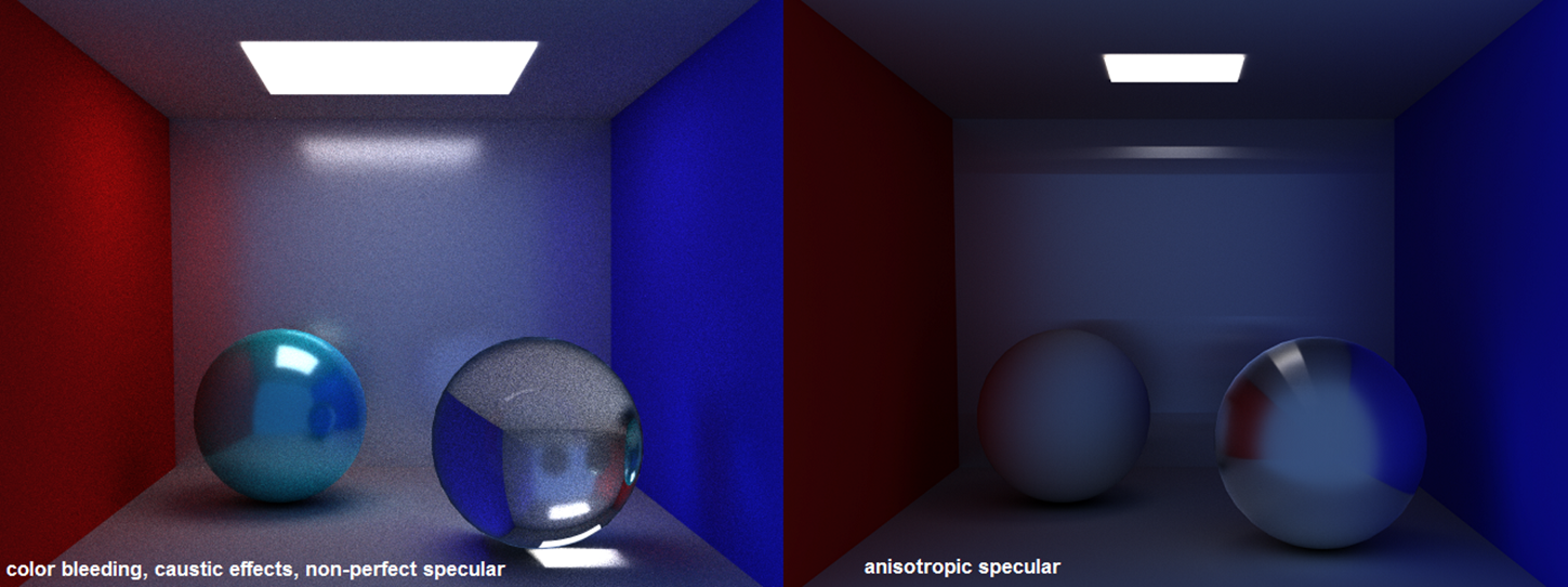
As a guarantee of its practical capability, our path tracer simulates the optical effects of all kinds of surface-to-surface reflection or refraction, not including the cases like polarized light or fluorescence which are rare in practice. For diffuse reflection, the Lambertian model adjusted by Ashikhmin and Shirley formula is used (Section 4.5) while Cook-Torrance microfacet model is responsible for specular or glossy reflection. Our path tracer also supports anisotropic material standardized by Wald model (Ward, 1992), which only modifies the Beckmann distribution factor in Cook-Torrance model (Cook & Torrance, 1982),
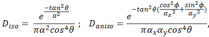
where
 and
and
 correspond to “roughness” of the material
in x and y direction w.r.t. tangent space. Taking azimuth angle
correspond to “roughness” of the material
in x and y direction w.r.t. tangent space. Taking azimuth angle
 as argument, it is easy to see that when
 the distribution is completely
determined by
and when
the distribution is completely
determined by
and when
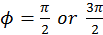 the distribution is totally decided by
.
the distribution is totally decided by
.
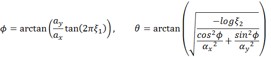
For importance sampling the Wald BRDF, two uniform unit random variables
 and
and
 are generated and it is easy to solve
the equations for azimuth angle
and altitude angle
are generated and it is easy to solve
the equations for azimuth angle
and altitude angle
 :
:
For surface-to-surface refraction, the Cook-Torrance microfacet model can be modified by recalculating the Jacobian matrix for the transform between half-vector and outgoing vector (Walter, Marschner, Li, Torrance, 2007), yielding
 , where D is the microfacet distribution
function (Beckmann in our implementation, G is the shadowing term (a
numerical approximation to Smith shadowing function in our
implementation, the roughness
coefficient
, where D is the microfacet distribution
function (Beckmann in our implementation, G is the shadowing term (a
numerical approximation to Smith shadowing function in our
implementation, the roughness
coefficient inside whom is substituted by 1/
 for anisotropic material) and J =
 , where
 are the index of refraction of the two
media, is the absolute value of the Jacobian matrix. The half-vector
in refraction indicates the normal of the sampled microfacet,
which can be obtained by calculating
are the index of refraction of the two
media, is the absolute value of the Jacobian matrix. The half-vector
in refraction indicates the normal of the sampled microfacet,
which can be obtained by calculating
 if BSDF needs to be determined from
arbitrary incoming and outgoing radiance so as in the case of multiple
importance sampling.
if BSDF needs to be determined from
arbitrary incoming and outgoing radiance so as in the case of multiple
importance sampling.
10.2 Volume Rendering
The rendering techniques so far are based on the assumption that spaces between surfaces are vacuum, which is only an effective simplification in ordinary cases with clear air. For phenomena like fog, smog, smoke, obvious scatter, absorption, and emission can happen between surfaces, which affect the radiance towards viewer. In the presence of such participating media, an integro-differential equation of transfer (Chandrasekhar, 1960) shows the directional radiance gradient of a point in participating media to model the change of radiance in space.
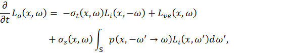
where
 is the point in space and
 is the direction in interest with
 being the measure of displacement along
the direction.
being the measure of displacement along
the direction.
 is the attenuation coefficient
accounting for both absorption and out-scattering, while
is the attenuation coefficient
accounting for both absorption and out-scattering, while
 is the scattering coefficient
controlling the magnitude of in-scattering, which has the phase function
is the scattering coefficient
controlling the magnitude of in-scattering, which has the phase function
 to define the probability density of
in-scattering from each direction.
to define the probability density of
in-scattering from each direction.
 and
and
 stand for media emission and incoming
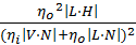
radiance, respectively. For isotropic media,
has a constant value of
stand for media emission and incoming
radiance, respectively. For isotropic media,
has a constant value of
 , which is intuitive as the integral of
differential angles in the sphere gives
, which is intuitive as the integral of
differential angles in the sphere gives
 . For general media, there is a phase
function developed by Henyey and Greenstein
(1941) which provides a simple asymmetry parameter
. For general media, there is a phase
function developed by Henyey and Greenstein
(1941) which provides a simple asymmetry parameter
 ranging from -1 to 1 to control the
“polarity” of the participating media.
ranging from -1 to 1 to control the
“polarity” of the participating media.
In practice, the integro-differential equation is solved by decomposing
different parts, calculating their values separately before using ray
marching to accumulate the values in each sample point on the incoming
ray. These sample points are treated as differential segments with
constant coefficients. Indeed, such numerical integration can be
estimated by Monte Carlo sampling. The parameter t of ray can naturally
be used as the measure of displacement along the ray direction.
Depending on the targeted convergence rate or frame rate, the step size
can be set larger or smaller. Normal Monte Carlo sampling would randomly
pick a point in each segment for radiance estimation. However, for
estimating the light transfer integral which is only one dimensional and
often has a smooth function, standard numerical integration may have an
edge over the Monte Carlo method. By using a stratified pattern (Pauly,
1999) which assigns same offset for each segment and randomizes the
offset for a new ray, it can be shown to have a lower variance than
Monte Carlo. The p.d.f. for such samples is also very simple, which is a
constant equal to the step size
 .
.
In the simplest case of volume rendering, where the participating media
has homogenous attributes, both emission and attenuation factors can be
directly evaluated by
 (where s is the length of the ray
segment of interest), which is the direct result of solving the
differential equation
(where s is the length of the ray
segment of interest), which is the direct result of solving the
differential equation
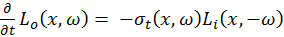 , also known as Beer’s law. If the
distribution of media density or other properties has an analytical
solution for such differential equation, the analytical solution (if it
is an elementary function) can be directly evaluated without using
sampling techniques, which is used where an analytical solution is
impossible, unknown, or too complex, or in the case where the
distribution is a customized discrete data set.
, also known as Beer’s law. If the
distribution of media density or other properties has an analytical
solution for such differential equation, the analytical solution (if it
is an elementary function) can be directly evaluated without using
sampling techniques, which is used where an analytical solution is
impossible, unknown, or too complex, or in the case where the
distribution is a customized discrete data set.
As mentioned before, the attenuation term and the augmentation term can be treated separately in computation, which maps well to the accumulation of mask and intermediate color in our implementation, expressed by
 ,
,
where
 is multiplied to the mask and
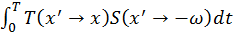 is estimated with samples and added to
the immediate color. Transmittance coefficient T can either be
analytically evaluated or estimated with samples as mentioned in
previous paragraph.
is estimated with samples and added to
the immediate color. Transmittance coefficient T can either be
analytically evaluated or estimated with samples as mentioned in
previous paragraph.
The sampling estimation of the augmentation term
can use the same stratified pattern
mentioned before to reduce the variance. However, inside
 , there is another integral which accounts
for in-scattering from all directions, the estimation of which is
another non-trivial task. For simplicity, we only consider single
scattering from direct lighting. A light sample can be taken as in next
event estimation and a shadow ray is shot from the current ray segment’s
sample point to the light to detect visibility. Note that this method
neglects the contribution from indirect lighting to the in-scattering,
which is often too weak to affect the rendering equality.
, there is another integral which accounts
for in-scattering from all directions, the estimation of which is
another non-trivial task. For simplicity, we only consider single
scattering from direct lighting. A light sample can be taken as in next
event estimation and a shadow ray is shot from the current ray segment’s
sample point to the light to detect visibility. Note that this method
neglects the contribution from indirect lighting to the in-scattering,
which is often too weak to affect the rendering equality.
It is worth mentioning that it is also possible to use metropolis light transport for sampling the in-scattering. A random number can be stored here for mutation in every frame so that directions with large contribution can be easily discovered and focused on, which is especially suitable for very anisotropic participating media.
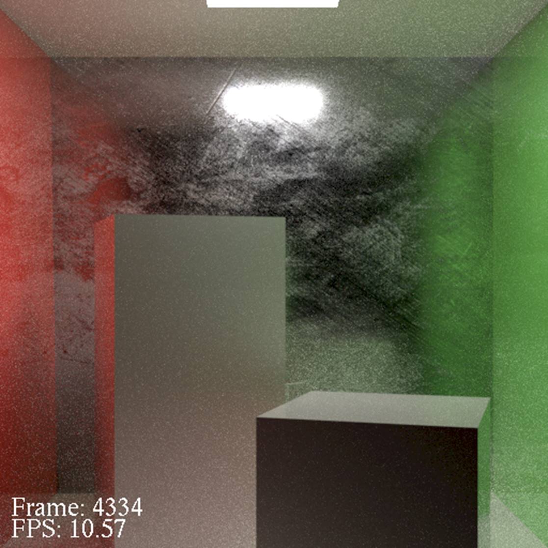
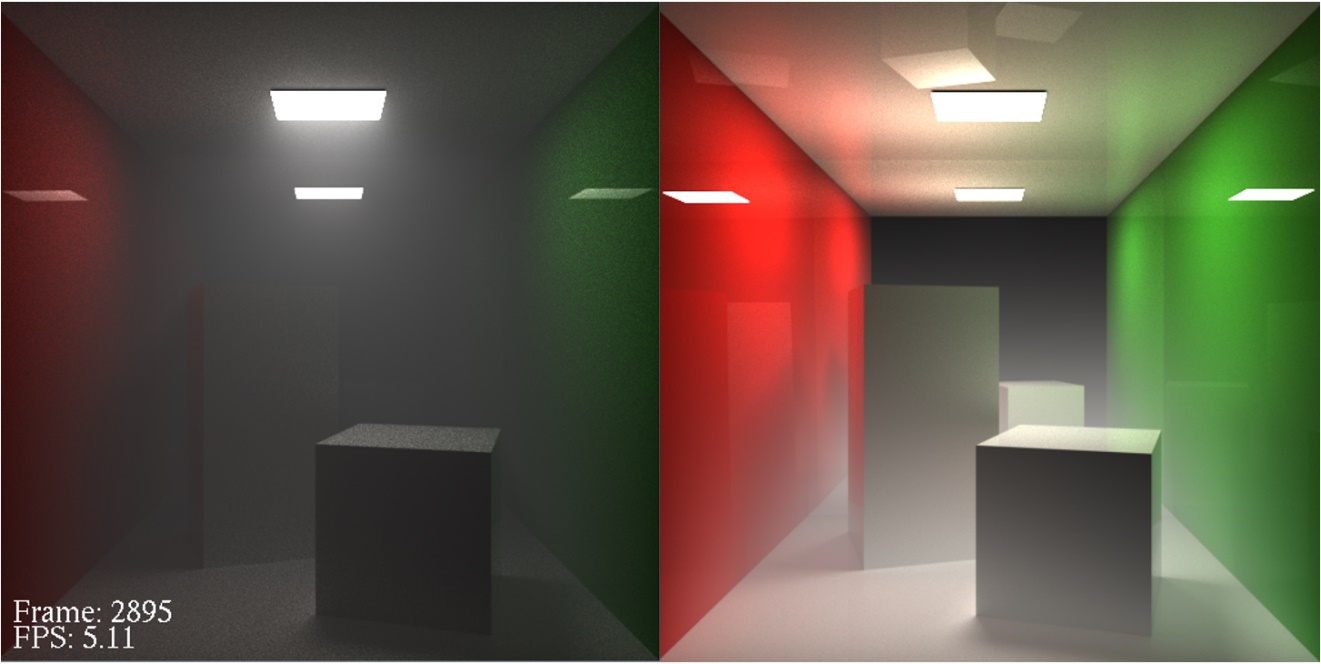
Two sample images are shown in Figure 11 to exhibit the visual effect of volume rendering. The first image shows strong scattering and absorption of light in a room with dense homogenous smog. The smog has a Henyey-Greenstein asymmetry parameter of 0.7, indicating that incident lights are primary scattered forward, as can be seen in the narrow shape of the illuminated cone under the area light. The second image illustrates fog with white emission and exponentially attenuated density in vertical direction, which is the miniature of the atmosphere in a box.
10.3 Subsurface Scattering
Scattering and absorption can happen inside objects as well. The reason for using BSDF to estimate the radiance from material is that many material can be categorized into metallic (which reflects most of the energy at surface) or dielectric which are either too opaque or too transparent to exhibit any obvious scattering effect. For material with an albedo high enough to be considered as non-transparent and not enough to be considered as opaque like jade, milk and skin, the effect of scattering inside cannot be ignored, for which BSDF cannot give sufficient approximation of the surface radiance. Instead, BSSRDF (bi-directional subsurface scattering reflectance distribution function) is used to include the contribution to the outgoing radiance of the point in interest from incoming radiance on other surface points. A 6-dimensional function
 (
( is known, the other 3 variables are all
2D) can be used to describe the sum of all radiance scattered from
is known, the other 3 variables are all
2D) can be used to describe the sum of all radiance scattered from
 to
in all possible paths. Again, to
calculate the outgoing radiance of the point in interest, one must
integrate the contribution from points all over the object surface,
which can be estimated by randomly sampling a surface point as a Monte
Carlo process. However, the BSSRDF itself is largely unknown due to the
complexity of the multiple scattering problem. Also, points in the
surrounding may contribute most of the radiance which implies that
indiscriminately choosing a surface point has an intolerably low
convergence rate.
to
in all possible paths. Again, to
calculate the outgoing radiance of the point in interest, one must
integrate the contribution from points all over the object surface,
which can be estimated by randomly sampling a surface point as a Monte
Carlo process. However, the BSSRDF itself is largely unknown due to the
complexity of the multiple scattering problem. Also, points in the
surrounding may contribute most of the radiance which implies that
indiscriminately choosing a surface point has an intolerably low
convergence rate.
To provide a practical approximation of general subsurface scattering, Jensen et al. introduced the dipole diffusion model (2001), which decomposes the BSSRDF into a diffusion term and a single scattering term as a simplification. Observing that the radiance distribution becomes nearly isotropic after thousands of scatterings in material with very high albedo like milk, they proposed a diffusion model that transforms the incoming ray into a dipole source and uses the radial diffusion profile of the material to compute the outgoing radiance. The diffusion term has an exponential falloff with respect to the distance from the incidence point, which provides an effective p.d.f. for importance sampling. Note that the key idea of this model is to interpolate between 2 extreme cases - pure single scattering and pure diffusion – for general material, which turns out to be an insufficient approximation when highly physically authentic pictures are required.
In our implementation, we only consider the contribution of the single
scattering term as a demonstration of the idea of subsurface scattering.
The program can be easily extended with an additional module for the
diffusion term estimation. Since single scattering only happens when the
refraction rays of
 and
and
 meet inside the material, BSSRDF is not
directly evaluated by taking a surface sample. Instead, after the ray
intersects the surface with BSSRDF component, a random distance is
generated by
meet inside the material, BSSRDF is not
directly evaluated by taking a surface sample. Instead, after the ray
intersects the surface with BSSRDF component, a random distance is
generated by
 , where
 is the unit uniform random variable and
 is the reduced scattering coefficient
corresponding to the tendency of forward scattering, followed by moving
the intersection point by such distance in the ray direction to become
the point of single scattering and using the phase function p to
importance sample the direction of scattering as the direction of the
next ray. Note that this method is only suitable for rendering
translucent objects with low to moderate albedo like jade. Objects with
high albedo still require at least the dipole model to render a
reasonable appearance.
is the reduced scattering coefficient
corresponding to the tendency of forward scattering, followed by moving
the intersection point by such distance in the ray direction to become
the point of single scattering and using the phase function p to
importance sample the direction of scattering as the direction of the
next ray. Note that this method is only suitable for rendering
translucent objects with low to moderate albedo like jade. Objects with
high albedo still require at least the dipole model to render a
reasonable appearance.
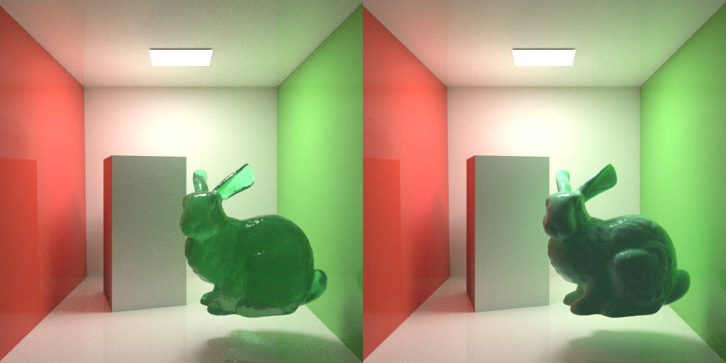
A pair of sample images are shown in Figure 12 to show the Stanford bunny with a deep jade color rendered as translucent and opaque material. The result of the translucent material shows the effect of subsurface single scattering. Note that thin parts of the object like the ear has a more acute response to the change of albedo.
10.4 Environment Map and Material Texture
As mentioned in the introduction, the heavy usage of textures can often
be found in rasterization based graphics used in most of the mainstream
video games. PBR workflow, as the de-facto industrial standard, uses a
variety of textures to describe the varying material attributes across
the texture space. Apart from the basic diffuse color texture or albedo
map, a roughness map is used to define the shape of the distribution of
normal in the microfacet model, such that the roughness value of 0
indicates a perfectly smooth surface point which only reflects at the
mirroring direction and the roughness value of 1 indicates a surface
point with almost equal amount of reflection in every direction which
makes it no longer look glossy. Similarly, a metalness map is used to
define the level of similarity to metal of each texel. A metalness value
of 1 defines a surface point that only has specular reflection with some
absorption of specific wavelengths which simulates the behavior of
metal, while a metalness value of 0 defines a completely dielectric
surface point that follows the Fresnel equation with real index of
refraction. More commonly, a uniform white specular color is defined for
every opaque object to substitute the evaluation of
 in the Fresnel equation when index of
refraction is not defined. Furthermore, a normal map is used to simulate
microscopic geometry for material with a complex surface texture and
ambient occlusion maps are used to compensate the corresponding effect
in the lack of global illumination in rasterization based graphics. For
still objects, light maps which baked the color bleeding or shadow
(requiring still light model) can be used in surrounding surfaces like
walls or floors to give a more realistic feeling of the rendering. Since
it is generally infeasible to generate real-time samples in
rasterization based graphics, usually an irradiance map and a
pre-filtered mipmap are precomputed from the environment map of the
scene to simulate diffuse and glossy reflection of indirect lighting
respectively.
in the Fresnel equation when index of
refraction is not defined. Furthermore, a normal map is used to simulate
microscopic geometry for material with a complex surface texture and
ambient occlusion maps are used to compensate the corresponding effect
in the lack of global illumination in rasterization based graphics. For
still objects, light maps which baked the color bleeding or shadow
(requiring still light model) can be used in surrounding surfaces like
walls or floors to give a more realistic feeling of the rendering. Since
it is generally infeasible to generate real-time samples in
rasterization based graphics, usually an irradiance map and a
pre-filtered mipmap are precomputed from the environment map of the
scene to simulate diffuse and glossy reflection of indirect lighting
respectively.
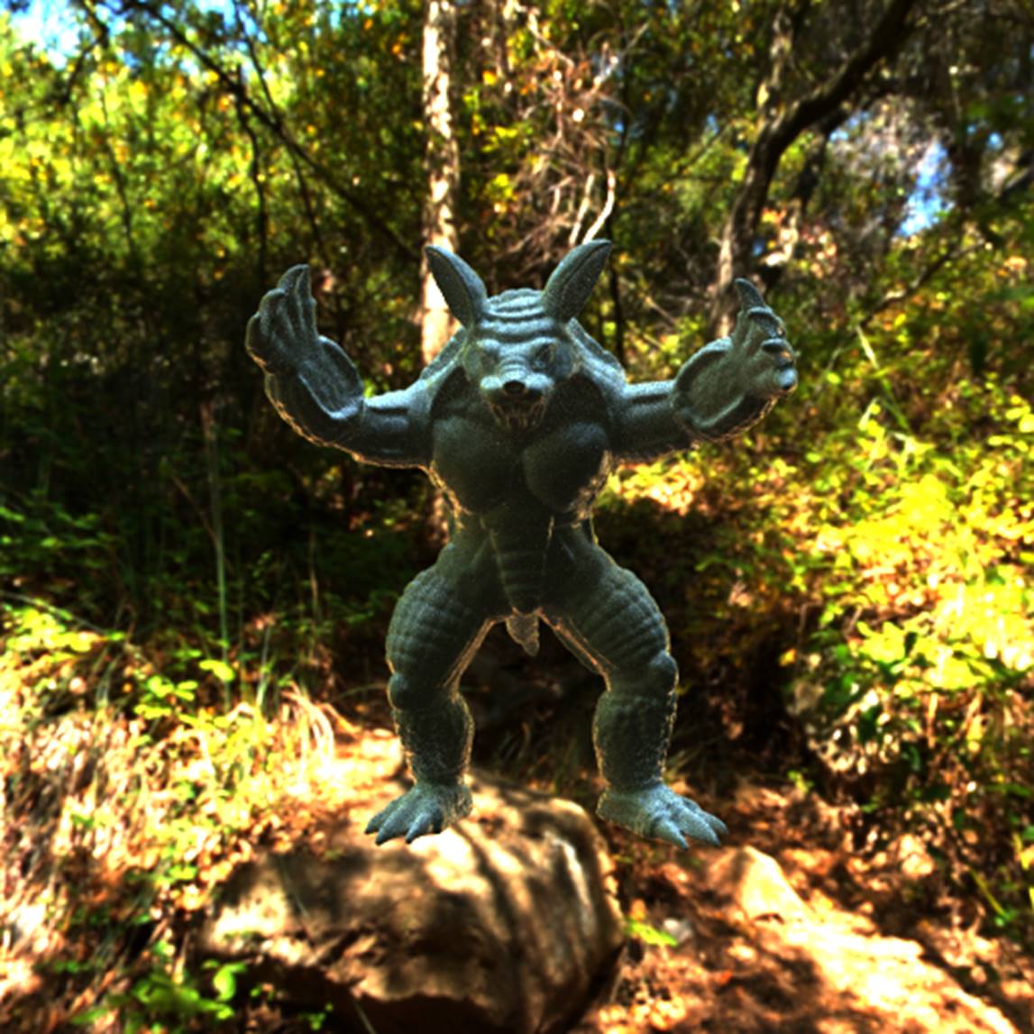
However, for path tracing, we only need the maps related to material attributes in texture space, i.e. albedo map, metalness map, and roughness map, because we are using a global illumination algorithm. We may also want to use environment maps as image-based lights – lighting from the outer environment like sky and sunlight are usually hard to be modeled as solid objects. Also, if the surrounding environment is sufficiently far, using environment map can avoid the ponderous task of modeling all objects from the border of the bounding environment to the point being shaded and accumulating all possible indirect lightings between any two objects. One can simulate the intricate indirect lighting effect by sampling the texel in the reflected ray direction if nothing in the local setting (the models in interest) is hit, treating the outer environment as an infinitely far sphere so that all rays can be seen as being shot from the center of the sphere. The environment map can either be stored as a cubemap or a spherical projection map. In our implementation, we use spherical projection maps due to easier computation and less chance of artefact.
Two sample images are shown in Figure 13 to demonstrate the effect of environment map as image based lighting and the material texture as surface attribute control. The second image simply provides albedo, roughness and metalness map to transform the diffuse back wall of the original Cornell box to a realistic scratched metal.