This post corrects some misconception in the former section [GAPT Series - 3] Path Tracing Algorithm as well as introduces some new rendering methods.
A key feature of path tracing that differentiates it with normal ray tracing is that it is a stochastic process (provided that the random numbers are real) instead of a deterministic process. Normal path tracing depends on Monte Carlo algorithm which gradually converges the result to the ground truth as the number of samples increases. Theoretically, one can uniformly sample all paths to converge to the correct result. However, given limited hardware resource and time requirement, we need to adapt the brute Monte Carlo algorithm by various strategies for different cases. The following sections will introduce the rendering equation we need to solve in path tracing and some most popular sampling methods.
9.1 BSDF and Importance Sampling
Importance sampling is an effective method for solving rendering
equation in high convergence rate. Basically, importance sampling
chooses samples by a designed probability density function and divides
the sample value by p.d.f. to return the result. If the designed p.d.f.
turns out to be proportional with the values, variance will be very low.
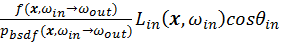
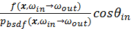
Since the sample value is determined by
 , both irradiance and BSDF decides the
p.d.f.
, both irradiance and BSDF decides the
p.d.f.
 of the surface sample. Importance
sampling BSDF is a more trivial task than importance sampling the
spatial distribution of incoming radiance. As long as a BSDF formula
(Lambertian, Cook-Torrance, Oren-Nayar, etc.) and corresponding surface
characteristics are provided, one can calculate
of the surface sample. Importance
sampling BSDF is a more trivial task than importance sampling the
spatial distribution of incoming radiance. As long as a BSDF formula
(Lambertian, Cook-Torrance, Oren-Nayar, etc.) and corresponding surface
characteristics are provided, one can calculate
 as the result. However, distribution of
 is harder to calculate in general case.
For indirect lighting on the surface point, it is impossible to know the
distribution of the incoming radiance, which is a chicken and egg
paradox. For direct lighting where
is harder to calculate in general case.
For indirect lighting on the surface point, it is impossible to know the
distribution of the incoming radiance, which is a chicken and egg
paradox. For direct lighting where
 , different methods can be applied to
find the p.d.f. With a simplified lighting model like point light or
area light, the distribution of incoming radiance is rather explicit.
However, when image-based lighting is used (e.g. environmental map or
sky box), advanced techniques are required to perform importance
sampling efficiently. The following sections will all focus in the case
of having explicit lighting models since it is easier to exemplify how
to utilize the p.d.f. of incoming radiance. Discussion for image-based
lighting will be continued in the next chapter. Since combing the effect
of two p.d.f. requires not only sampling on the surface point, but the
lighting model or lighting image as well. A technique called multiple
importance sampling will be introduced in Section 9.3.
, different methods can be applied to
find the p.d.f. With a simplified lighting model like point light or
area light, the distribution of incoming radiance is rather explicit.
However, when image-based lighting is used (e.g. environmental map or
sky box), advanced techniques are required to perform importance
sampling efficiently. The following sections will all focus in the case
of having explicit lighting models since it is easier to exemplify how
to utilize the p.d.f. of incoming radiance. Discussion for image-based
lighting will be continued in the next chapter. Since combing the effect
of two p.d.f. requires not only sampling on the surface point, but the
lighting model or lighting image as well. A technique called multiple
importance sampling will be introduced in Section 9.3.
9.2 Next Event Estimation
For direct lighting with explicit model, lighting computation can be
directly done without shooting ray to the lights, which is called next
event estimation. Literally, it accounts for the contribution of what
may happen in the next iteration. For ideal diffuse surface, whose BSDF
is spatial uniform (usually expressed by Lambertian model), this task is
very simple. One only needs to sample a point in one of the lights. Take
diffuse area light (emission of a point is uniform in all directions) as
an example, if the emission across the light emission surface is the
same, one only needs to uniformly sample the shape of the light.
Otherwise, usually there is an existing intensity distribution to use.
After that, to convert the area measure of p.d.f to solid angle measure,
from formula
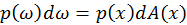 (Veach, 1997) we can derive
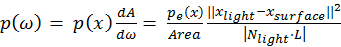 , which can be used as the p.d.f for
incoming radiance. Given that Lambertian surface has a BSDF of
, which can be used as the p.d.f for
incoming radiance. Given that Lambertian surface has a BSDF of
 , the final color can be expressed in the
simple formula
, the final color can be expressed in the
simple formula
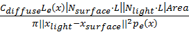 .
.
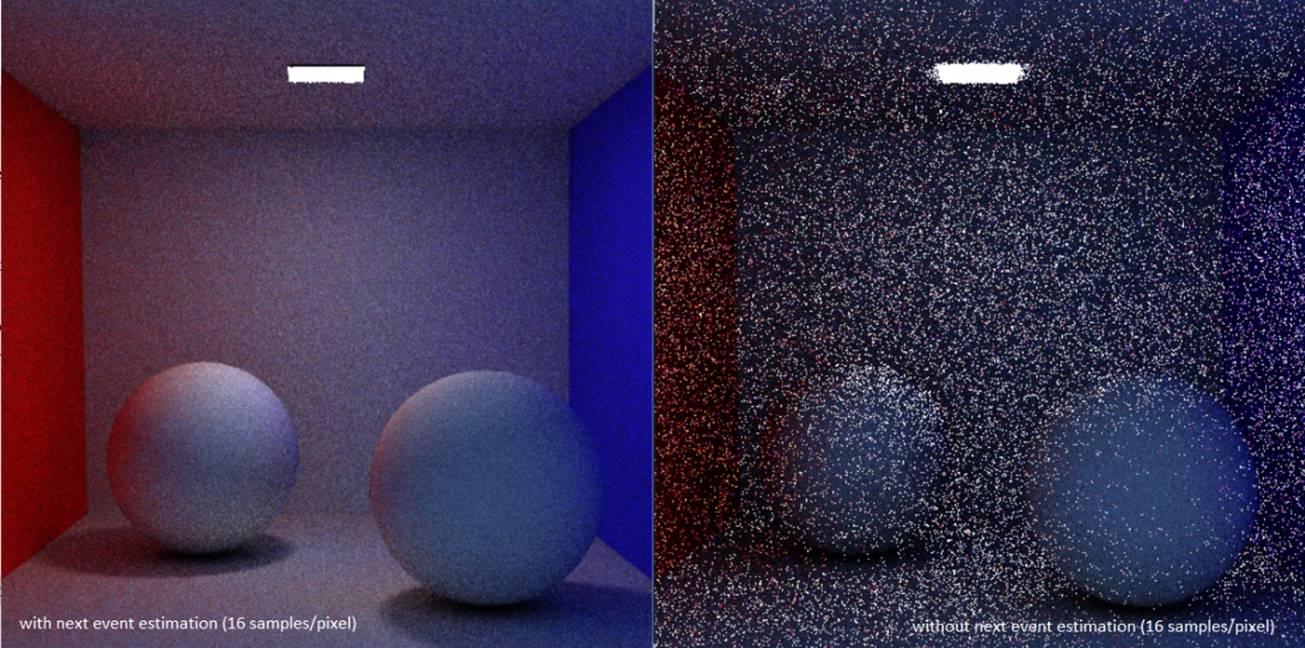
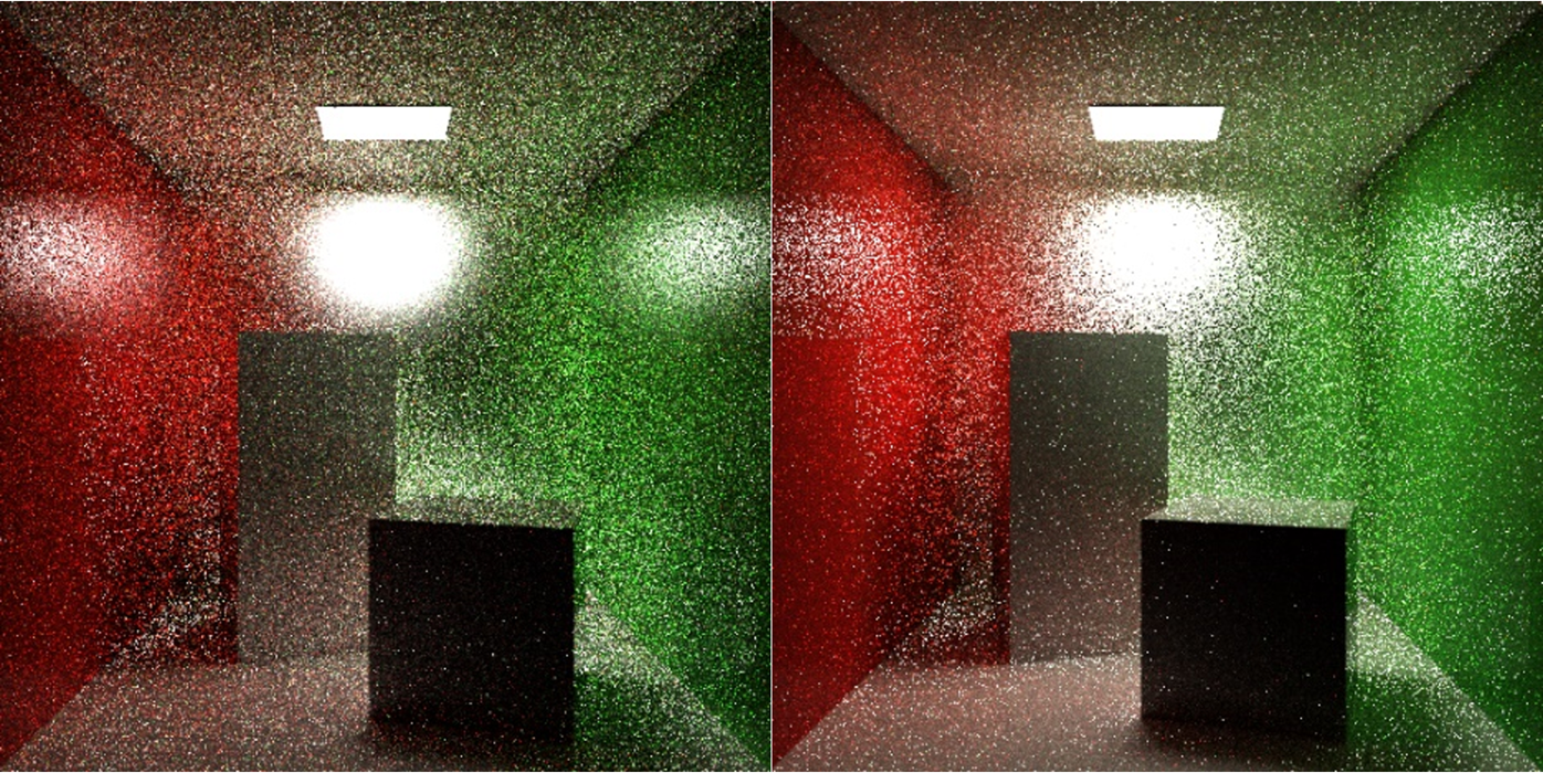
For diffuse area lights of simple geometric shape like triangle, uniform sampling can be trivially done by using barycentric coordinates. Apart from light sampling, we also need to shoot a shadow ray from the surface point being shaded to the sampled light point. Since ray-triangle intersection test is a bottleneck in ray tracing for reasonably complex scenes, this means we will almost halve the frame rate. However, the benefit of next event estimation totally worth the costs it takes. Figure 5 is an example picture comparing the convergence rate of diffuse reflection of two balls under highlight with and without next event estimation, where 16 samples are taken for each pixel for both sampling methods. Although the frame rate for rendering with next event estimation is only 60% of that without next event estimation, the noise level of the former is dramatically lower than the latter.
However, this example only shows the case where the shaded surface has a uniform BSDF. For surfaces with general non-uniform BSDF like glossy surface in the Cook-Torrance microfacet model, sampling the light is inefficient for variance reduction. An extreme case is the perfect mirror reflection, whose BSDF is a delta function. Since only the mirrored direction of the view vector w.r.t the surface normal contributes to the result, sampling from a random point in the light model has zero probability to contribute. We would naturally want to sample according to the BSDF. A general case is, a glossy surface whose BSDF values concentrate in a moderately small range and the lighting model occupies moderately large portion of the hemisphere around the surface being shaded. As a rescue for general cases, multiple importance sampling will be introduced later. However, if we want to have a balance between quality and speed, next event estimation can be mixed with direct path tracing for different BSDF components. Especially for the case of surface material with only diffuse and perfectly specular reflection, doing a next event estimation by multiple importance sampling would be redundant. Instead, if the BSDF component in current iteration is diffuse, we will set a flag to avoid counting in the contribution if we hit a light in next iteration. Otherwise, such flag will have a false value, allowing the radiance of the light hit by the main path to be accounted into. For determining which BSDF component to sample, we will use a “Fresnel switch”, which will be introduced in the next section.
9.3 Fresnel Switch and The Russian Roulette
Physically, there are only reflection and refraction when light as an
electromagnetic wave interacts with a surface, the ratio of which is
determined by the media’s refractive indices in two sides of the surface
and the incidence angle of the light. The original formula is actually
different for s and p polarization component in the light ray. However,
in computer graphics, we normally treat the light as non-polarized.
Under this assumption, Schlick’s approximation (Schlick, 1994) can be
used to calculate the Fresnel factor:
 . However, in the standard PBR workflow,
the refractive index is usually only provided for translucent objects.
Although we can look up for the refractive index of many kinds of
material, for metals and semiconductors, the refractive index n is a
complex number, which complicates the calculation. Since the refractive
index of the metal indicates an absorption of the color without
transmission, specular color is used to approximate the reflection
intensity in normal direction. In practice, there is usually an albedo
map and a metalness map for metallic objects. The metalness of a point
determines the ratio in interpolation between white color and albedo
color. In the case of metalness equal to 1, the albedo color will become
the specular color in reflection, as what we refer to as the color of
metal actually suggests how different wavelengths of light is absorbed
rather than transmitted or scattered in the case for dielectric
material.
. However, in the standard PBR workflow,
the refractive index is usually only provided for translucent objects.
Although we can look up for the refractive index of many kinds of
material, for metals and semiconductors, the refractive index n is a
complex number, which complicates the calculation. Since the refractive
index of the metal indicates an absorption of the color without
transmission, specular color is used to approximate the reflection
intensity in normal direction. In practice, there is usually an albedo
map and a metalness map for metallic objects. The metalness of a point
determines the ratio in interpolation between white color and albedo
color. In the case of metalness equal to 1, the albedo color will become
the specular color in reflection, as what we refer to as the color of
metal actually suggests how different wavelengths of light is absorbed
rather than transmitted or scattered in the case for dielectric
material.
Briefly, if there is an explicit definition of index of refraction, we
will use that for
 calculation of the material. Otherwise,
we interpolate the albedo color provided in material map or scene
description file with the white specular color meaning complete
reflection of light according to the metalness of the material, as
defined in normal PBR workflow. However, considering the fact that
dielectric material also absorbs light to some degree, the specular
color can be attenuated by some factor less than 1 to provide a more
realistic appearance.
calculation of the material. Otherwise,
we interpolate the albedo color provided in material map or scene
description file with the white specular color meaning complete
reflection of light according to the metalness of the material, as
defined in normal PBR workflow. However, considering the fact that
dielectric material also absorbs light to some degree, the specular
color can be attenuated by some factor less than 1 to provide a more
realistic appearance.
After
 is calculated, we can calculate the
Fresnel factor by substituting the dot product of view vector and the
surface normal into the Schlick’s formula. Notice that there is a power
of 5, which is better calculated by brute multiplication of 5 times than
using the pow function in the C++ or CUDA library for better
performance. The Fresnel factor R indicates the ratio of reflection. In
path tracing, this indicates the probability of choosing the specular
BRDF to sample for the next direction. Complementarily, T = 1 – R
expresses the probability of transmission.
is calculated, we can calculate the
Fresnel factor by substituting the dot product of view vector and the
surface normal into the Schlick’s formula. Notice that there is a power
of 5, which is better calculated by brute multiplication of 5 times than
using the pow function in the C++ or CUDA library for better
performance. The Fresnel factor R indicates the ratio of reflection. In
path tracing, this indicates the probability of choosing the specular
BRDF to sample for the next direction. Complementarily, T = 1 – R
expresses the probability of transmission.
In our workflow, diffuse reflection is also modeled as a transmission,
which will immediately be scattered back by particles beneath the
surface uniformly in all directions, which is usually modeled by
Lambertian BSDF. However, to be more physically realistic, we can refer
to Ashikhmin and Shirley’s model (2000) which models the surface as one
glossy layer above and one diffuse layer beneath with infinitesimal
distance between. The back scattering in realistic diffuse reflection
happens at the diffuse layer as a Lambertian process, after which the
reflected ray is attenuated again by transmitted across the glossy
surface, implying less contribution of next ray in near tangent
directions. For energy conservation, Ashikhmin and Shirley also include
a scaling constant
 in the formula. Therefore, the complete
BSDF is :
in the formula. Therefore, the complete
BSDF is :
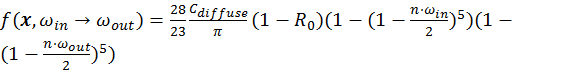 .
.
Russian roulette is used to choose the BSDF component given the Fresnel factor and other related material attributes. If the generated normalized uniform random number is above the Fresnel threshold R, next ray will be transmission or diffuse reflection. Again, the “translucency” attribute of the material will be used as the threshold for determining transmission or diffuse reflection, which is actually an approximation of general subsurface scattering, which will be discussed in next chapter. The Fresnel switch guarantees we can preview the statistically authentic result in real-time. However, the thread divergence implies a severe time penalty in GPU. Suggestion will be given in the SIMD optimization analysis in Chapter 6.
The Russian Roulette is also responsible for thread termination. Since
any surface cannot amplify the intensity of incoming light, the RGB
value of the mask
( ) is always less than or equal to 1. The
intensity of the mask (which is the value of the largest component of
RGB, or the value in HSV decomposition of color) is then used as the
threshold to terminate paths. To be statistically correct, the mask is
always divided by the threshold value after the Russian Roulette test,
which is a very intuitive process – if the reflectance of the surface is
weak, early termination with value-compensated masks is equivalent to
multiple iterations of normal masks. Such termination decision greatly
speeds up rendering without increasing the variance.
) is always less than or equal to 1. The
intensity of the mask (which is the value of the largest component of
RGB, or the value in HSV decomposition of color) is then used as the
threshold to terminate paths. To be statistically correct, the mask is
always divided by the threshold value after the Russian Roulette test,
which is a very intuitive process – if the reflectance of the surface is
weak, early termination with value-compensated masks is equivalent to
multiple iterations of normal masks. Such termination decision greatly
speeds up rendering without increasing the variance.
For generating photorealistic result, it is possible to use the Russian Roulette solely to determinate termination without setting a maximum depth. However, considering the extreme case where the camera is inside an enclosed room and all surfaces are perfectly specular and reflect all lights, there is still a need to set a maximum depth.
9.4 Multiple Importance Sampling
Returning to our question of next event estimation or direct lighting
computation for general surface BSDF, the technique called multiple
importance sampling was introduced by Eric Veach in his 1997’s PhD
dissertation. Basically, it uses a simple strategy to provide a highly
efficient and low-variance estimate of a multi-factor integral mapped to
a Monte Carlo process where two or more sampling distributions are used,
usually in different sampling domains. Given an integral
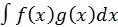 with two available sampling distributions
 and
and
 , a simple formula given to as the Monte
Carlo estimator
, a simple formula given to as the Monte
Carlo estimator
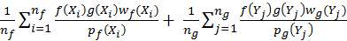 , where
 and
and
 are number of samples taken for each
distribution and
are number of samples taken for each
distribution and
 and
and
 are specially chosen weighting functions
which must guarantee that the expected value of the estimation equals
the integral
. As expected, the weighting functions can
be chosen from some heuristics to minimize the variance.
are specially chosen weighting functions
which must guarantee that the expected value of the estimation equals
the integral
. As expected, the weighting functions can
be chosen from some heuristics to minimize the variance.
Veach also offers two heuristic weighting functions: balance heuristic
and power heuristic. In a general form
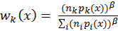 where k is any particular sampling
method, balance heuristic always takes
where k is any particular sampling
method, balance heuristic always takes
 = 1 while power heuristic gives the
freedom to choose any exponent
. Veach then uses numerical tests to
determine that
= 1 while power heuristic gives the
freedom to choose any exponent
. Veach then uses numerical tests to
determine that
 is a good value for most cases.
In order to verify the practical result of multiple importance sampling and the effect of the choice of weighting function, some test cases were performed and sample images of the results are listed below.
The first test case compares the result of multiple importance sampling (both from BSDF and light) and single importance sampling (only from BSDF). In each frame, a path is traced for each pixel. Although rendered only 10 frames, the MIS result clearly displays the shape of the reflection of the strong area light on the rough mirror behind the boxes and its further reflection on the alongside walls. In contrast, the non-MIS result generated by 100 frames still has a very noisy presentation of the reflected shape of the highlight. Note that for reflection on the floor and ceiling, which has a low roughness, non-MIS in frame 100 still has a lower noise level than that of MIS in frame 10. Since most contribution to the color comes from samples generated from BSDF, the strength of multiple importance sampling diminishes, which is also the case when the BSDF is near uniform.
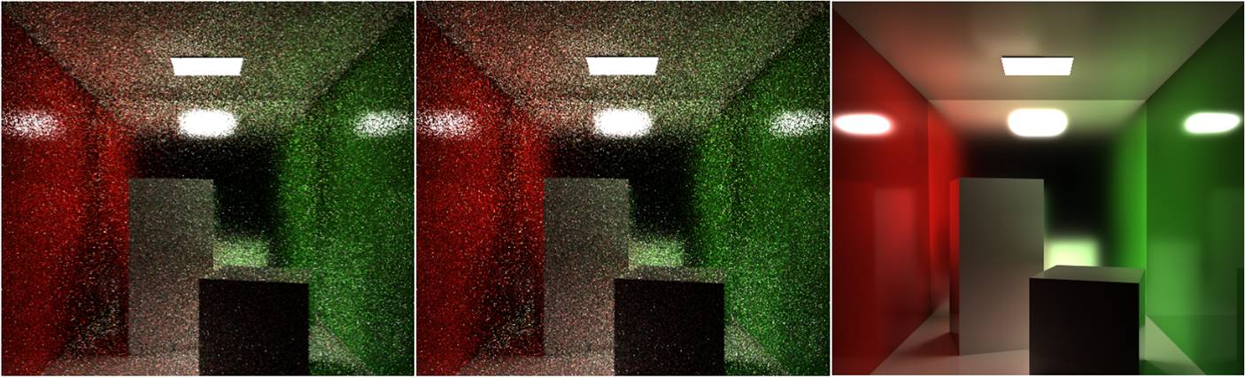
Another test case aims at comparing the effect of balance heuristic and power heuristic. The images in Figure 7 above show the result of rendering the same Cornell box scene with moderately rough back mirror in 10 frames for both methods. Without very carefully inspecting the images, it is nearly impossible to observe any difference between two images. However, noise level is indeed lower when using power heuristic. Intuitively, if one carefully looks at some dark regions in the picture like the front face of the shorter box, an observation that many noise points are brighter in the image generated by balance heuristic (Since both cases use the same seed for random number generation, it is possible to compare noise point at same pixel position). However, we also offer numerical analysis to compare the percentage of difference between the two images and the ground truth (rendered by metropolis light transport in 80000 frames). The result of calculating the histogram correlation coefficient with the ground truth for each image shows that image generated by power heuristic has a value of 0.7517, larger than the image generated by balance heuristic which has a value of 0.7488. Although this is only a minor difference, it proves that power heuristic indeed has lower variance.
9.5 Bi-directional Path Tracing
An important fact of the sampling methods we have discussed so far is that the variance level depends on both geometry of the emissive surfaces or lights and the local geometry of surrounding surfaces. For brute path tracing, the rate of hitting the background (out of the scene) will be much larger than hitting the light if the summed area of lights is too small or lights are almost locally occluded, which results in only a few of terminated rays would carry the color of emission, causing large variance. For importance sampling or multiple importance sampling, shadow rays must be shot to the light. Expected variance level can only be guaranteed when the chance of misses is of the same order of magnitude as that of chance of hits; otherwise, the variance level will degenerate to that of brute path tracing. Thankfully, this problem can be solved by also shooting a ray from the light and “connect” the end vertices of the eye path and light path to calculate the contribution, which is called bi-directional path tracing (Lafortune & Willems, 1993).
The core problem in bi-directional path tracing is the “connect”
process. Since the contribution of incoming radiance is sampled as a
point (end vertex of light path) in the area domain, we must convert
that to the solid angle domain to obtain the result. The
 term in the rendering equation can be
converted to an equivalent
term in the rendering equation can be
converted to an equivalent
 in the domain of all surface areas,
where
in the domain of all surface areas,
where
 is the visibility factor which equals to
1 if the connection path is not occluded and 0 otherwise and
is the visibility factor which equals to
1 if the connection path is not occluded and 0 otherwise and
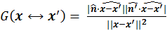 is the geometry term.
Importantly, we not only connect the terminated end points of light path and eye path, but the intermediate path ends as well. However, since each connection involves a ray-triangle intersection test, performance will be greatly affected - for path lengths of O(n), there will be O(n^2^) intersection tests. In some situation like perfect mirror reflection, we can exclude the contribution of light path since it has a zero probability as a way to save computation time. It is worth mentioning that for all combinations with a specific path length, the contribution of each should be divided by the total number of combinations to maintain energy conservation. For any combined path length of n, there are n + 1 ways of combination of eye path and light path if we want to include the contribution of all kinds of combination. It is also possible to apply importance sampling here as a specific path combination can be weighted by the p.d.f. in all path combinations of the same length. However, that requires additional space to store the intermediate results and may not be good for GPU performance. Next event estimation can also be applied here, so that direct lighting component exists in all combined path length less than or equal to (maximum eye path length + 1), for which the denominator of contribution should be incremented by 1 to include this factor.
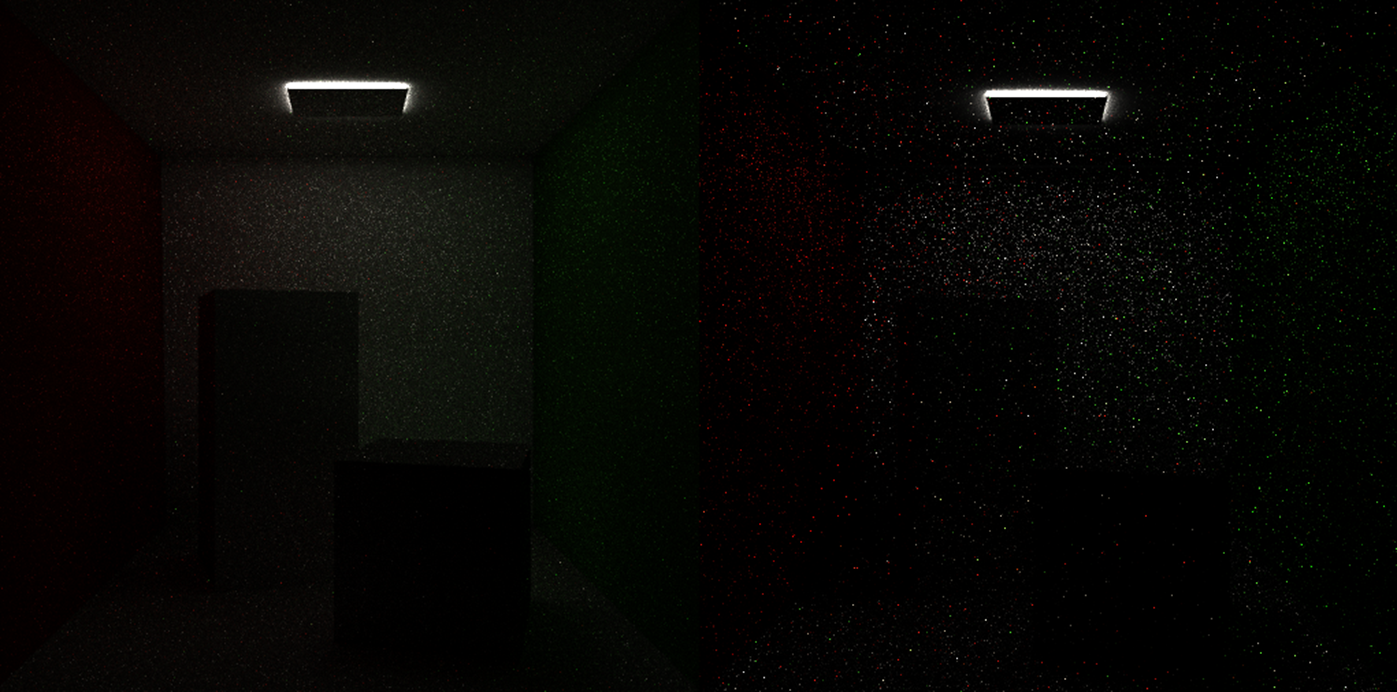
In order to test the effect of bi-directional path tracing, we simply inverted the light in the original Cornell Box scene such that light faces the ceiling and the light can only bounce to other surfaces via the small crevices on the rim of the light. The sample image in Figure 8 shows that both rendered in 100 frames, bi-directional path remarkably reduces the noise level comparing to that when only using next event estimation, totally worth for the reduction of frame rate to 50%.
9.6 Metropolis Light Transport
Using multiple importance sampling and bi-directional path tracing, it
is still difficult to maintain low variance in integration estimation
for solving problems like bright indirect light, caustics caused by
reflected light from caustics and light coming from long, narrow, and
tortuous corridors. The key problem of previous sampling methods is that
they only consider local importance (light or surface BSDF) rather than
the importance of the whole path. In terms of global importance
sampling, the original Monte Carlo method is still a brute force
solution. To our rescue, there is a rendering algorithm called
Metropolis Light Transport (MLT) adapted from the Metropolis–Hastings
sampling algorithm based on the Markov Chain Monte Carlo (MCMC) method
(Veach, 1997). It has the nice feature that the probability of a path
being sampled corresponds to its contribution in the global integral of
the radiance toward camera and such paths can be locally explored by
designing some mutation strategy. Basically, it proposes new
perturbation or mutation to current path in every iteration and accepts
the proposal with a probability
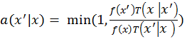 , where the
 and
and
 are the radiance values and
 and
and
 are tentative transition functions which
indicate the probability density of transforming from a state to another
state in the designed mutation strategy. In general cases,
and
are not equal. For example, given the
specific task of sampling caustics, we can define a mutation strategy
that only moves the path vertices at the specular surface. As a return,
such mutation can have a transitional probability corresponding with
local p.d.f. – if such point
are tentative transition functions which
indicate the probability density of transforming from a state to another
state in the designed mutation strategy. In general cases,
and
are not equal. For example, given the
specific task of sampling caustics, we can define a mutation strategy
that only moves the path vertices at the specular surface. As a return,
such mutation can have a transitional probability corresponding with
local p.d.f. – if such point
 in a specular surface contributes more
highlight than another
in a specular surface contributes more
highlight than another
 in the same surface as its BSDF
suggests, the probability of moving from
in the same surface as its BSDF
suggests, the probability of moving from
 to
to
 is greater than moving from
to
, giving
is greater than moving from
to
, giving
 . However, different mutation strategies
need to be designed in different kinds of task in order to achieve the
highest rendering quality. For general kinds of task, we can ignore
local p.d.f. in mutation while still maintaining a good performance. A
way of doing so is to store and mutate only the random numbers for every
samples generated in the path (selecting camera ray, choosing next ray
direction, picking points on area light, determining Russian roulette
value, etc.), which will function as “global-local” perturbations on
current path, as suggested by Pharr & Humphreys (2011).
. However, different mutation strategies
need to be designed in different kinds of task in order to achieve the
highest rendering quality. For general kinds of task, we can ignore
local p.d.f. in mutation while still maintaining a good performance. A
way of doing so is to store and mutate only the random numbers for every
samples generated in the path (selecting camera ray, choosing next ray
direction, picking points on area light, determining Russian roulette
value, etc.), which will function as “global-local” perturbations on
current path, as suggested by Pharr & Humphreys (2011).
Another issue for MLT is ergodicity (Veach, 1997). The MCMC process must traverse the whole path space without getting stuck at some subspaces, which turns out to have a solution of setting a probability for large (global) mutation. Each iteration will test a random number against the threshold. If, for example, the random number is lower than the threshold 0.25, it means on average there is 1 large mutation and 3 small (local) mutations out of 4 mutations. The local mutations are sampled by an exponential distribution (Veach, 1997), implying much larger chance of less movement from the original place while allowing moderately large local mutations. The global mutations are sampled uniformly across the [0,1] interval.
Still another problem of MLT is that in order to choose a probability density function p corresponding to the radiance contribution of the path, which is a scalar, we must find a way to map the 3D radiance value to 1D space to determine the acceptance probability. A reasonable way of doing this is using the Y value in XYZ color space which reflects the intensity perceived by human eye. A simple conversion formula is given as Y = 0.212671R + 0.715160G + 0.072169B. Note that no matter what mapping formula is chosen, the result is still unbiased. Choosing a mapping closer to eye perception curve allows faster convergence and better visual appearance in same number of iterations.
Nevertheless, another important issue of MLT is the start-up bias
(Veach, 1997). Considering the estimation function
 , where f is the radiance, p is the
mapped intensity and w is the lens filter function. The
Metropolis–Hastings algorithm guarantees that the sampling probability
, where f is the radiance, p is the
mapped intensity and w is the lens filter function. The
Metropolis–Hastings algorithm guarantees that the sampling probability
 in equilibrium, giving the minimal
variance. However, we have no way to sample in such
in equilibrium, giving the minimal
variance. However, we have no way to sample in such
 before equilibrium is reached but
gradually converge to the correct p.d.f, even though we use
before equilibrium is reached but
gradually converge to the correct p.d.f, even though we use
 as the denominator which is actually not
the real p.d.f. for current sample. This causes incorrect color in first
few samples, known as start-up bias. Depending on the requirement, if
the rendering task is not time-restrictive or not aimed for dynamic
scene, we can just discard the first few samples until the result become
reasonable. Using a smaller large mutation rate is also a remedy for
start-up bias. However, tradeoffs are that complex local paths become
harder to detect and while the global appearance converges quickly,
local features like caustics and glossy reflection emerge very slowly.
In practice, if the scene contains mostly diffuse surfaces, large
mutation rate can be set larger. On the other hand, if the intricate
optical effects are the emphasis of rendering, large mutation rate
should be set much smaller. In fact, designing specific mutation
strategies with customized transition functions may be better than just
using “global-local” mutations.
as the denominator which is actually not
the real p.d.f. for current sample. This causes incorrect color in first
few samples, known as start-up bias. Depending on the requirement, if
the rendering task is not time-restrictive or not aimed for dynamic
scene, we can just discard the first few samples until the result become
reasonable. Using a smaller large mutation rate is also a remedy for
start-up bias. However, tradeoffs are that complex local paths become
harder to detect and while the global appearance converges quickly,
local features like caustics and glossy reflection emerge very slowly.
In practice, if the scene contains mostly diffuse surfaces, large
mutation rate can be set larger. On the other hand, if the intricate
optical effects are the emphasis of rendering, large mutation rate
should be set much smaller. In fact, designing specific mutation
strategies with customized transition functions may be better than just
using “global-local” mutations.
It turns out that MLT can be trivially mapped to GPU by running independent tasks in each thread, as is implemented by this project. However, such method still has its defects. For decent convergence rate, the number of threads is set to be equal to the number of screen pixels (so that for the average case, every pixel can be shaded in every frame), which implies high space complexity, due to stored random numbers (stored as float) in graphic memory. If the screen width and height are W and H, maximum path length (or combined path length if bi-directional path tracing is used) is k and about 10 samples need to be generated for each path segment (as in our implementation), there will be 40k*W*H bytes in total for storing the MLT data. With 1920*1080 resolution and a reasonable k = 30, there will be 2.37G of data, exceeding size of the graphic memory for many low to mid end graphic cards nowadays. To solve this issue, some data compression can be done and it is also possible to let the threads collaborate in a more efficient way, which means running less number of tasks while keeping same or lower variance. However, we will not study this topic in this project due to the effectiveness of existing performance and existence of other important issues.
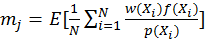
Last but not least, the estimation of global radiance
 (||x|| indicates a measure of the
magnitude of intensity of the RGB color) at the beginning will affect
the overall luminance of the final result. From the formula
,
(||x|| indicates a measure of the
magnitude of intensity of the RGB color) at the beginning will affect
the overall luminance of the final result. From the formula
,
 is chosen to be
 , yielding
 as the radiance contribution from one
sample,
where
as the radiance contribution from one
sample,
where functions as a scaling factor for all
samples. As a result, in the case where the rendered result is required
to be physically authentic, more sample should be taken to estimate the
global radiance, although it causes a considerable overhead.
functions as a scaling factor for all
samples. As a result, in the case where the rendered result is required
to be physically authentic, more sample should be taken to estimate the
global radiance, although it causes a considerable overhead.
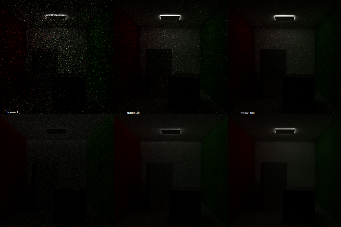
To illustrate the advantage of MLT, some sample image from tests are shown in Figure 9. In both cases, bi-directional path tracing with multiple importance sampled direct lighting is used; the first row shows the result in frame 1, 30, 100 for normal Monte Carlo (MC) sampling whereas the second row shows the results at same frames for MLT. Reader will notice difference of the ways of the two estimators accumulate color. While maintaining a low noise level from the initial frame, MLT estimator exhibits start-up bias as shown by the dim color of the part of the ceiling directly illuminated by the light. In frame 100, the MLT estimator almost reaches the equilibrium as observed in comparison with the MC estimator with respect to color of directly illuminated part of the ceiling. It is worth mentioning that such level of variance is can only be achieved in frame number > 1000 by MC estimator while the MLT estimator is only slightly slower than MC estimator, cause of which mainly attributes to the atomic memory write as each thread runs an independent MLT task which can write color to all pixels on the screen.